Difference between revisions of "MainPage:Nuclear:Summer2017:Blessed"
| (38 intermediate revisions by 2 users not shown) | |||
| Line 6: | Line 6: | ||
<h1> Introduction </h1> | <h1> Introduction </h1> | ||
<p> | <p> | ||
| − | Lead | + | Lead Tungstate crystals have been found to be very effective in particle energy measurements and thus, the continuous developments in nuclear physics. |
This is because the crystals have have favorable properties such as: | This is because the crystals have have favorable properties such as: | ||
| Line 21: | Line 21: | ||
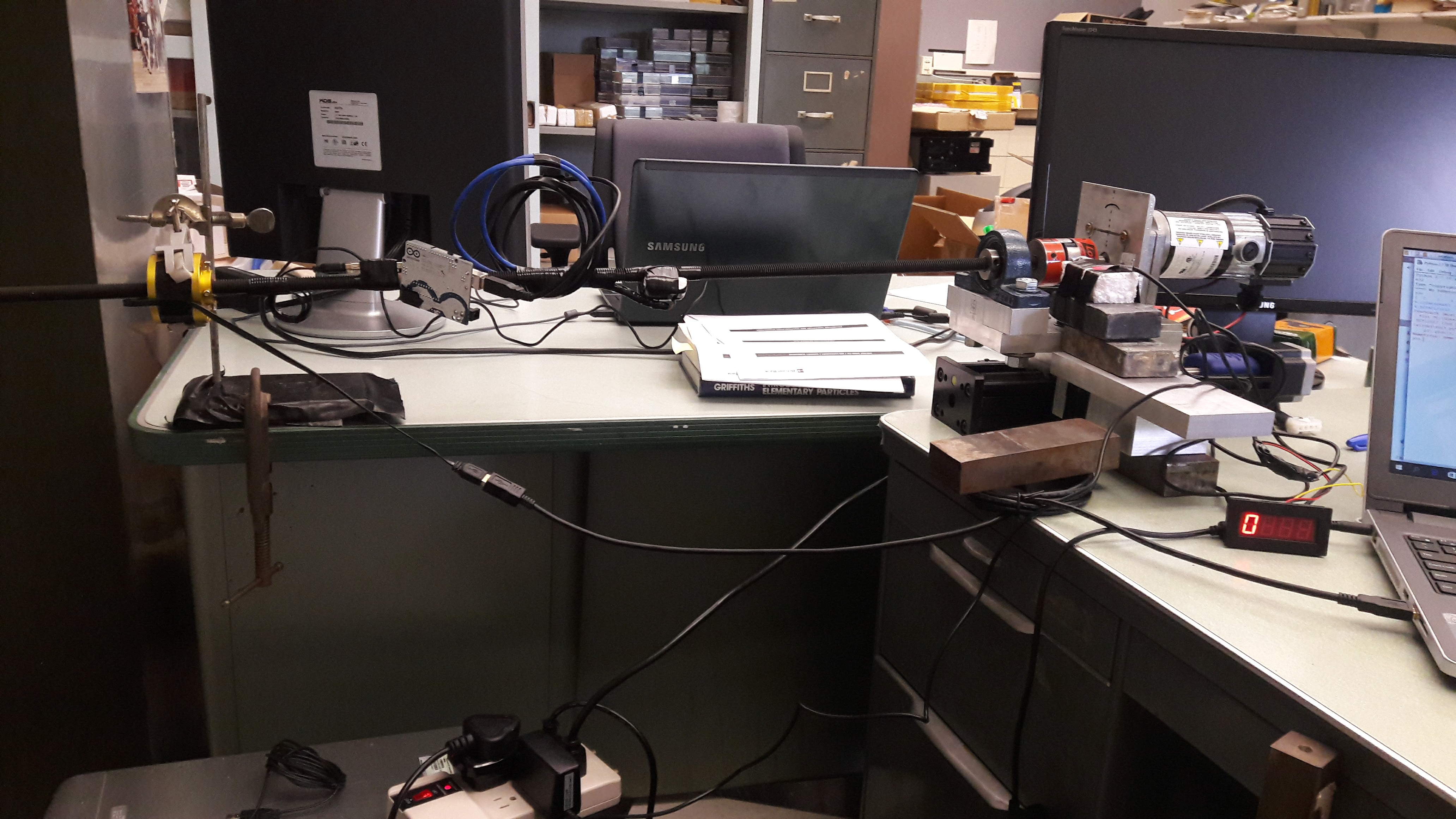
<h1> Description of the crystal drawing apparatus </h1> | <h1> Description of the crystal drawing apparatus </h1> | ||
| − | <p> | + | <p> |
| + | [http://www.vsl.cua.edu/cua_phy/images/0/0d/20170705_142352.jpg Mechanical setup (horizontally)] | ||
| − | <h1> Calibration of the accelerometer </h1> | + | [[File:20170705_142352.jpg|thumb|center|250px| Mechanical setup (horizontally)]] |
| − | <p> | + | |
| + | [[File:20170712_153623.jpg|thumb|center|250px| Mechanical setup (vertically)]] | ||
| + | </p> | ||
| + | |||
| + | |||
| + | |||
| + | <h1>Calibration of the accelerometer:</h1> | ||
| + | <p> | ||
| + | The accelerometer measures proper acceleration and can be calibrated using known values of the gravitational acceleration on the surface of the earth. We connect the Arduino board to the accelerometer as can be seen from the following figure and we allow the accelerometer to draw its input voltage from the output of the digital output pins cause it uses very little current. | ||
| + | |||
| + | [[File:20170705_014739.jpg|thumb|center|250px| An illustration of how the wires should be connected between the Arduino board and the ADXL3xx accelerometer. The top one is the accelerometer.]] | ||
| + | |||
| + | Due to the high sensitivity of the accelerometer, we have to attach it to a heavy metal to ensure that it doesn't move. To do this, the accelerometer was placed inside a ............ then taped to an iron metal block as can be seen in the figure below. Now, the problem that arise here is that this block was uneven and this tilted the accelerometer by different angles for different orientations. A gravity linear....... was used to measure the length of the sides which were then used to calculate the angle of tilt. | ||
| − | |||
| − | |||
[[File:20170621 135238.jpg|thumb|center|250px| Initial setup to calibrate the accelerometer]] | [[File:20170621 135238.jpg|thumb|center|250px| Initial setup to calibrate the accelerometer]] | ||
| − | + | The next step is to collect results after attaching the set-up to a laptop. To do this, some software and programming is required. The code for the arduino board can be found here............ and it measures readings from all 3-axes of the accelerometer. Arduino prints out the output values from each axis to the screen and we need a software that will print these values to a file saved on a computer. For this reason, Gobetwino was installed. Gobetwino is ................. Data needs to be collected with all 3-axes aligned and anti-aligned with gravity with the equipment stationery. The plot below shows the values measured by the accelerometer vs time and we can see that they are constant which is parallel to the fact that gravitational acceleration is constant near the surface of the earth. | |
| + | |||
| + | [[File:figx.png|thumb|center|250px| Accelerometer reading vs time for the x-axis]] | ||
| + | |||
| + | [[File:figy.png|thumb|center|250px| Accelerometer reading vs time for the y-axis]] | ||
| + | |||
| + | [[File:figz.png|thumb|center|250px| Accelerometer reading vs time for the z-axis]] | ||
| − | + | To analyse the data, VPython was used. We know that the measurement of the accelerometer is proportional to the acceleration signal and so, a linear model/relation would be appropriate here such that ACCELERATION = A*SIGNAL + B. Here A and B are constants which will be determined as follows: let SIGNAL be the average of the values measured by the accelerometer and let ACCELERATION be +9.8(gravity) when gravity is aligned with the +axis and -9.8 when gravity is anti-aligned with the -axes then solve the following equations. | |
| − | + | +9.8 = A*+SIG + B | |
| − | + | -9.8 = A*-SIG + B | |
| + | |||
| + | Calibration needs to be done separately for different axis. The code that was used to obtain these constants can be found here...... for the x-axis and it's error, similarly, you can find A and B for the y and z axis with the errors. Uncertainties were obtained from using the angle of tilt that was mentioned earlier. The results of the calibration are tabulated below: | ||
| + | |||
| + | |||
| + | <table style="width:100%"> | ||
| + | <Table border ="5"> | ||
| + | |||
| + | <tr> | ||
| + | <th> </th> | ||
| + | <th>X</th> | ||
| + | <th>Y</th> | ||
| + | <th>Z</th> | ||
| + | </tr> | ||
| + | <tr> | ||
| + | <td>A</td> | ||
| + | <td>-0.14767501</td> | ||
| + | <td>-0.14689038</td> | ||
| + | <td>-0.14759584</td> | ||
| + | </tr> | ||
| + | <tr> | ||
| + | <td>B</td> | ||
| + | <td>49.83232499</td> | ||
| + | <td>49.28610738</td> | ||
| + | <td>51.09182802</td> | ||
| + | </tr> | ||
| + | <tr> | ||
| + | <td>Misalignment angle</td> | ||
| + | <td>2.26 degrees</td> | ||
| + | <td>2.11 degrees</td> | ||
| + | <td>1.89 degrees</td> | ||
| + | </tr> | ||
| + | <tr> | ||
| + | <td>Deviation percentage</td> | ||
| + | <td>0.08 %</td> | ||
| + | <td>0.07 %</td> | ||
| + | <td>0.05 %</td> | ||
| + | </tr> | ||
| + | </table> | ||
| + | |||
| + | |||
| + | [[File:vib2aa.png|thumb|center|250px| Acceleration vs time for all the axis when the system is steady to see the vibrational effects. First 19 seconds are with stable cables and the rest are with cables moving around]] | ||
| + | |||
| + | [[File:vib2b.png|thumb|center|250px| Acceleration vs time for all the axis when the system is steady to see the vibrational effects. First 19 seconds are with stable cables and the rest are with cables moving around]] | ||
| − | |||
| − | |||
<h1> Rotation Studies </h1> | <h1> Rotation Studies </h1> | ||
| − | <p> | + | <p> |
| + | Before we can look into the vibrations of the system, we need to characterize the rotation of the system. I used a tachometer, which consisted of two magnets, one attached to the rotating rod and one stationary as close as possible to the rotating one, yet not coming into contact. This can be seen below: | ||
| + | |||
| + | [[File:20170705_123402.jpg|thumb|center|250px| Tachometer attached to a magnet with a second magnet attached to coupling hubs to measure the speed of rotations]] | ||
| + | |||
| + | The aim is to have our rod rotating at 35rpm and the tachometer helps with that. Since the cabling is attached to the rod, the cables entangle when it rotates. To avoid these issues with cabling in a rotating system I installed a slip ring and signal conditioner in the setup. The slip ring had to be clamped to ensure that it doesn't move, this can be seen in the section on the apparatus. To construct a reproducible way to set the rotation speed, I fitted the data using a linear model and determined the DC motor setting that will produce a rotation of 35rpm. This setting is 6.93 with a standard error of 0.36. The figure below shows the fit. | ||
| + | |||
| + | [[File:rot2.png|thumb|center|250px| Comparing each setting of the rotation equipment to the corresponding speed and approximating the data with a linear model]] | ||
| + | </p> | ||
| + | |||
| + | |||
| + | |||
| + | |||
| + | <h1> Vibration Studies </h1> | ||
| + | <p> | ||
| + | As mentioned in the introduction, we need to damp the system so that the vibrations don't affect the highly sensitive temperature gradient of the mixture. Now, we will determine the amount of vibrations that are introduced to our set-up by the rotation using the accelerometer and by taking data at different sampling rates and rotation speeds around the required 35rpm. Three sampling rates were used(100ms, 10ms and 1ms) and these can be changed on the Arduino code on the delay() function. A problem arises with the software due to memory for small sampling rates and this can be countered by increasing the baud rate on the Arduino and Gobetwino software and switching off the status messages and command output on Gobetwino. We will quantify the vibrations with the system lying horizontally and then vertically(which will be the case for the final setup). | ||
| + | |||
| + | |||
| + | |||
| + | <h3>Horizontal orientation </h3> | ||
| + | This orientation is such that the coordinate system has the z-axis and x-axis getting to be parallel with gravity during the rotation, while the y-axis is parallel to the shaft, thus perpendicular to gravity always. | ||
| + | |||
| + | |||
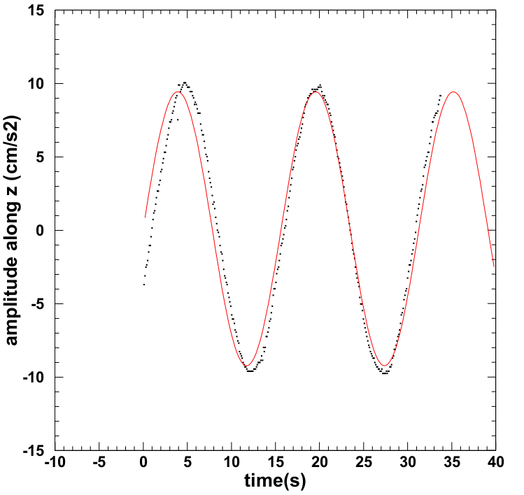
| + | The three figures below show the acceleration for a sampling rate of 100ms and different rotation speeds | ||
| + | |||
| + | [[File:vib2c.png|thumb|center|250px| Acceleration vs time for a rotation with a speed of 2rpm]] | ||
| + | |||
| + | |||
| + | [[File:Vib1.png|thumb|center|250px| Initial result using the calibrated accelerometer sensor and the assembled mechanical setup of the crystal drawing prototype. The coordinate system is such that the z-axis and x-axis get to be parallel with gravity, while the y-axis is parallel to the shaft. The sampling rate was 100ms and the rotation with a speed of 10rpm]] | ||
| + | |||
| + | [[File:vib2d.png|thumb|center|250px| Acceleration vs time for a rotation with a speed of 16rpm]] | ||
| + | |||
| + | [http://www.vsl.cua.edu/cua_phy/images/7/75/Vibparm.png Example of Vibration parametrization] | ||
| + | |||
| + | [http://www.vsl.cua.edu/cua_phy/images/b/b3/Fft_vib2acc.png Example of FFT] | ||
| + | </p> | ||
| + | |||
| + | <h3>Vertical orientation</h3> | ||
| + | This orientation is such that the y-axis lies parallel to gravity with the -y-axis in the direction of gravity, while the x-axis and z-axis are always perpendicular to gravity. For this orientation, we will only analyse different sampling rates at a speed of 35rpm. The results can be seen below, first for the steady states(no rotation) then for the 35rpm: | ||
| + | |||
| + | [[File:vibvcs2.png|thumb|center|250px| Acceleration vs time for a the steady state]] | ||
| + | |||
| + | [[File:vibvcr2a.png|thumb|center|250px| Acceleration vs time for a rotation with a speed of 35rpm and a sampling rate of 1ms]] | ||
<h1> Calibration of the load cell </h1> | <h1> Calibration of the load cell </h1> | ||
| − | <p> | + | <p>To determine the weight of the growing crystal, a load cell needs to be attached to the rod. I constructed a test setup with a Futek load-cell and it needed to be calibrated beforehand. In calibrating the load cell, I used standard weights ranging from 1g to 1125g and a SENSIT test and measurement software for readout. This setup can be seen below: |
| + | |||
| + | [[File:20170706_155523.jpg|thumb|center|250px| Load-cell calibration, standard weights hanging from a load cell though a string and a mass holder]] | ||
| + | |||
| + | Using different masses, readings were collected and the plots below show the data points fitted with a linear model as well as the deviations of the experimental values. | ||
| + | The equation of the fit is given by: Force = 49.7822582681*reading + 0.0369811029 with a standard error of 0.0291704541. | ||
| + | |||
| + | [[File:load3.png|thumb|center|250px| Load-cell calibration, fitted experimental data]] | ||
| + | |||
| + | [[File:load3b.png|thumb|center|250px| Load-cell calibration, fitted experimental data zoomed in to show the small error bars]] | ||
| + | |||
| + | The resolution of the load cell is of order of 1*10**(-9) but its precision is of the order of 1*10**(-3). We can determine the crystal's mass gain per unit time using m = density*Velocity_of_liquid*Area_of_cylinder. The density of our mixture is 8.3g/cm3, we pull the rod up at 3mm/hr, we can assume a crystal of diameter 40mm and length of 5mm. Plugging into the above, we get 78.23g/hr??????????????Quite large! | ||
| + | |||
| + | The crystal growth rate is in grams so the resolution associated with the load-cell is higher and this means that it will be sufficient for our purposes. | ||
| + | </p> | ||
Latest revision as of 16:22, 18 July 2017
Commissioning of a crystal drawing system
Abstract
Text.
Introduction
Lead Tungstate crystals have been found to be very effective in particle energy measurements and thus, the continuous developments in nuclear physics. This is because the crystals have have favorable properties such as:
1.Relatively high light yield:
2.Small Moliere radius:
This is a constant/property of a material which gives the scale of the transverse dimension of the fully contained electromagnetic showers(initiated when a high-energy electron, positron or photon enters a material resulting in either the photoelectric effect, Compton scattering or pair production. All this depends on the energy of the primary particle.) It can simply be defined as the radius of a cylinder containing an average of 90% of the shower's energy deposition.
3.Short radiation length:
This is the mean distance that a high-energy particle travels before losing 1/e of its energy by bremsstrahlung. One would expect that this distance be dependent on the energy of the particle but it only depends on the mass number and atomic number of the material.
However, manufacturing of Lead-Tungsten crystals has yet to be perfected and there has been considerate variation in the properties of the produced crystals. In this project, we aim to build a prototype for the manufacturing of these crystals locally by the Czochralski method. In building this prototype, the behaviour of the mechanical set-up is critical due to the sensitivity introduced by the above method. During the process of making the crystals, the rod needs to be rotated at 35rpm in order to maintain a sufficient mixture of the melt. So that it doesn't fall back into crucible? This rotation introduces some vibrations into the system, along the vibration of the surface the set-up is on or the building in general.
Description of the crystal drawing apparatus
Mechanical setup (horizontally)


Calibration of the accelerometer:
The accelerometer measures proper acceleration and can be calibrated using known values of the gravitational acceleration on the surface of the earth. We connect the Arduino board to the accelerometer as can be seen from the following figure and we allow the accelerometer to draw its input voltage from the output of the digital output pins cause it uses very little current.

Due to the high sensitivity of the accelerometer, we have to attach it to a heavy metal to ensure that it doesn't move. To do this, the accelerometer was placed inside a ............ then taped to an iron metal block as can be seen in the figure below. Now, the problem that arise here is that this block was uneven and this tilted the accelerometer by different angles for different orientations. A gravity linear....... was used to measure the length of the sides which were then used to calculate the angle of tilt.

The next step is to collect results after attaching the set-up to a laptop. To do this, some software and programming is required. The code for the arduino board can be found here............ and it measures readings from all 3-axes of the accelerometer. Arduino prints out the output values from each axis to the screen and we need a software that will print these values to a file saved on a computer. For this reason, Gobetwino was installed. Gobetwino is ................. Data needs to be collected with all 3-axes aligned and anti-aligned with gravity with the equipment stationery. The plot below shows the values measured by the accelerometer vs time and we can see that they are constant which is parallel to the fact that gravitational acceleration is constant near the surface of the earth.


To analyse the data, VPython was used. We know that the measurement of the accelerometer is proportional to the acceleration signal and so, a linear model/relation would be appropriate here such that ACCELERATION = A*SIGNAL + B. Here A and B are constants which will be determined as follows: let SIGNAL be the average of the values measured by the accelerometer and let ACCELERATION be +9.8(gravity) when gravity is aligned with the +axis and -9.8 when gravity is anti-aligned with the -axes then solve the following equations.
+9.8 = A*+SIG + B
-9.8 = A*-SIG + B
Calibration needs to be done separately for different axis. The code that was used to obtain these constants can be found here...... for the x-axis and it's error, similarly, you can find A and B for the y and z axis with the errors. Uncertainties were obtained from using the angle of tilt that was mentioned earlier. The results of the calibration are tabulated below:
| X | Y | Z | |
|---|---|---|---|
| A | -0.14767501 | -0.14689038 | -0.14759584 |
| B | 49.83232499 | 49.28610738 | 51.09182802 |
| Misalignment angle | 2.26 degrees | 2.11 degrees | 1.89 degrees |
| Deviation percentage | 0.08 % | 0.07 % | 0.05 % |


Rotation Studies
Before we can look into the vibrations of the system, we need to characterize the rotation of the system. I used a tachometer, which consisted of two magnets, one attached to the rotating rod and one stationary as close as possible to the rotating one, yet not coming into contact. This can be seen below:

The aim is to have our rod rotating at 35rpm and the tachometer helps with that. Since the cabling is attached to the rod, the cables entangle when it rotates. To avoid these issues with cabling in a rotating system I installed a slip ring and signal conditioner in the setup. The slip ring had to be clamped to ensure that it doesn't move, this can be seen in the section on the apparatus. To construct a reproducible way to set the rotation speed, I fitted the data using a linear model and determined the DC motor setting that will produce a rotation of 35rpm. This setting is 6.93 with a standard error of 0.36. The figure below shows the fit.

Vibration Studies
As mentioned in the introduction, we need to damp the system so that the vibrations don't affect the highly sensitive temperature gradient of the mixture. Now, we will determine the amount of vibrations that are introduced to our set-up by the rotation using the accelerometer and by taking data at different sampling rates and rotation speeds around the required 35rpm. Three sampling rates were used(100ms, 10ms and 1ms) and these can be changed on the Arduino code on the delay() function. A problem arises with the software due to memory for small sampling rates and this can be countered by increasing the baud rate on the Arduino and Gobetwino software and switching off the status messages and command output on Gobetwino. We will quantify the vibrations with the system lying horizontally and then vertically(which will be the case for the final setup).
Horizontal orientation
This orientation is such that the coordinate system has the z-axis and x-axis getting to be parallel with gravity during the rotation, while the y-axis is parallel to the shaft, thus perpendicular to gravity always.
The three figures below show the acceleration for a sampling rate of 100ms and different rotation speeds


Example of Vibration parametrization
Vertical orientation
This orientation is such that the y-axis lies parallel to gravity with the -y-axis in the direction of gravity, while the x-axis and z-axis are always perpendicular to gravity. For this orientation, we will only analyse different sampling rates at a speed of 35rpm. The results can be seen below, first for the steady states(no rotation) then for the 35rpm:


Calibration of the load cell
To determine the weight of the growing crystal, a load cell needs to be attached to the rod. I constructed a test setup with a Futek load-cell and it needed to be calibrated beforehand. In calibrating the load cell, I used standard weights ranging from 1g to 1125g and a SENSIT test and measurement software for readout. This setup can be seen below:

Using different masses, readings were collected and the plots below show the data points fitted with a linear model as well as the deviations of the experimental values. The equation of the fit is given by: Force = 49.7822582681*reading + 0.0369811029 with a standard error of 0.0291704541.


The resolution of the load cell is of order of 1*10**(-9) but its precision is of the order of 1*10**(-3). We can determine the crystal's mass gain per unit time using m = density*Velocity_of_liquid*Area_of_cylinder. The density of our mixture is 8.3g/cm3, we pull the rod up at 3mm/hr, we can assume a crystal of diameter 40mm and length of 5mm. Plugging into the above, we get 78.23g/hr??????????????Quite large!
The crystal growth rate is in grams so the resolution associated with the load-cell is higher and this means that it will be sufficient for our purposes.